The Kelly Criterion, which we covered in a previous article, estimates what fraction of risk capital to use for a particular bet in order to maximise the long-term wealth expectation. We know also that it does not consider the risk to be financially wiped out along the way. This is why risk-of-ruin is an indicator that so greatly complements it. In this article, we will present a numerical method to calculate it and run through examples on how it can be used to conservatively size bets.

Formal definition

What is commonly called risk-of-ruin can be defined as the probability for risk capital to fall to or below a certain percentage of its initial value when taking the same bet a set number of times and putting every time, the same percentage of remaining capital at risk. As its definition suggests, it takes two parameters: the ruin level, a number between 0.0 and 1.0 which we will note \( H \) and the maximum number of bets which is a positive integer expressed as \( N \). It could be written in mathematical form as:

$$ \mathbb{R}(H,N;f,b,p) = \mathbb{Pr} \left[ \min_{i \in 0..N} C(i) \leq H \right] $$

where \( C(i) \) is the remaining risk capital after the i-th bet, \( p \) is the probability of winning the bet, \( b \) is the win/loss ratio (or net-fractional-odds in Kelly’s framework) and \( f \) the fraction of capital to be waged. This formal definition does not seem trivial to solve analytically, so how can risk-of-ruin be calculated?

Binomial tree approach

Since a common bet has two possible outcomes, a series of the same bet putting at risk the same fraction of the portfolio can be modelled as a recombining binomial tree. Here is an illustration of the tree for a series of two bets:

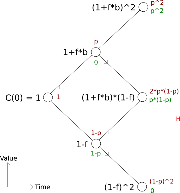
The capital level at each node is in a black font while the probability of attaining the node if the ruin level was 0 is in brown. For a ruin level different than zero, the probability assigned to some nodes would change because of the possibility of early stoppage: if the ruin event is triggered before the last bet, the experiment stops thereby influencing the probability of all the subsequent nodes that could have otherwise been visited. For the ruin level represented by the red line, this particular processing generates the final probabilities displayed in green. The risk-of-ruin is then the sum of the final probability of all the nodes falling below the ruin level (1-p in our example).

This numerical method can be implemented fairly easily in the programming language of your choice. Here is a demo of this algorithm as a web service. Its outputs were checked against those of a Monte-Carlo simulator as anyone should do to test their code. Now that we have a way of calculating it, how can we intuitively interpret the number?

The intuition behind the number

In order to get a “feel” for the risk-of-ruin measure, let’s consider a set of bets that all have the same expected value \( E \), but a different set of win rate \( p \) and win/loss ratio \( b \). In this set, all bets have characteristics that satisfy the following equation:

$$ p = \frac{1+E}{1+b} $$

Here, it is clear that the larger the number \( b \), the smaller the number \( p \). Let’s plot the risk of ruin as a function of the net-fractional-odds of the bet for a wager of 3%, an expected profit of 5%, a ruin level of 50% and a maximum number of bets of 100:

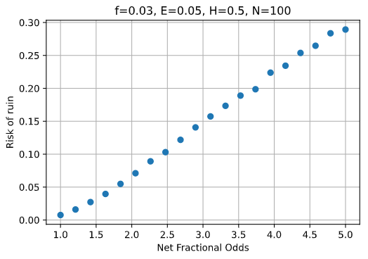
The risk-of-ruin clearly increases with the net-fractional-odds number, which in our setting means that the risk-of-ruin decreases as the win rate increases. Intuitively, this is merely confirming a suspicion: The lower the probability of a loss per bet, the less we should get worried about compounded losses over time. Now how can we use it to manage bet size?

Application to bet sizing

Since risk-of-ruin is a coherent way of comparing the long-term risk of a bet policy, it can be used to evaluate the inherent risk for one bet size over another. The idea is to consistently use a wager size that keeps the risk-of-ruin equal to a certain value. For example, setting a ruin level at 50% and a maximum number of bets of 100, we can derive the appropriate wager for any bet encountered that generates a risk-of-ruin of 5%. Here is a table showing a comparison of this approach with Kelly’s:

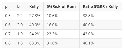
The table clearly shows that bet sizing using this method is way more conservative than by following the Kelly criterion. Both are not exactly proportional but not completely far off. The choice of ruin level, maximum number of bets and target risk-of-ruin are left for the speculator to choose. They should be set based on his/her own risk appetite.

Conclusion

Risk-of-ruin is a more flexible and coherent approach to bet sizing than using a fixed fraction of the Kelly Criterion. Calculating its exact value for a single bet is more complex but very manageable using numerical methods. When facing multiple simultaneous bets, we would however need to switch to a Monte-Carlo approach to derive it effectively, which would be a dent on performance.

If you like this post, don’t forget to follow me on Twitter and get notified of the next publication.