After collecting the backtest data from your latest systematic trading system, the final step is to decide whether or not the strategy is fit to be used in a live setting. Subjectively, there are a range of indicators that could be looked into to take the final decision. Here we will consider one that is based around the observed average return-per-trade. It is a particularly interesting approach as it allows us to derive the probability for the strategy to have an edge.

Chances for the strategy to have an edge

A strategy is said to have an edge simply when it is expected - in a statistical sense - to generate a profit. Mathematically, if we define a variable \( X_{\pi} \) as the return given by a trade generated by the strategy \( pi \), we can write that the strategy \( pi \) has an edge if:

$$ \mathbb{E}(X_{\pi}) > 0 $$

Practically, a value for this expectation can only be estimated empirically from historical test data. A non-biased estimator is the average of all return-per-trade \( x_i \) observed over our sample dataset. If we note \( \hat{E} \) our sample estimator for the expectation, we can express it as :

$$ \hat{E} = \frac{1}{N} \sum_{i=1}^{N} x_i $$

So, if our average return-per-trade is positive then the burning question is whether or not this sample estimate is a reliable guess for the expectation quantity we are after. This can be achieved by quantifying the probability for the actual expectation to be greater than zero given the sample estimate. If we call the probability for our strategy to have an edge \( p_e \), it can be written as:

$$ p_e = \mathbb{Pr} [ \mathbb{E} \left( X \right) > 0 ] $$

Naive Bootstrapping

In statistics, a common method to generate a distribution for a sample estimate is to use bootstrapping. The general idea of the approach is to simulate sample sets from the original observed set and derive a distribution of the estimator based on these newly generated sample values. The assumption inherent to this method is that the observed samples are representative of the measured random variable. This means that the larger the original sample set the more representative the bootstrapping result can potentially be.

There are several methods that can generate a new sample set from the original one. The simplest method is to build new sets of the same size as the original by randomly choosing with replacement individual samples from the original set. Once an empirical density is generated for our expectation estimator, we can calculate the probability of interest by fitting to a parametrised distribution or simply by counting occurrences. Let’s run through an example to see the method in action.

Real world example

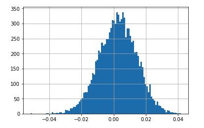
Based on the backtest results of an algorithmic strategy (roughly 3k trades), 10k estimator values were collected using a naive bootstrapping method. Here are the results in an histogram format:

The shape of this density function is very close to a Normal distribution as the QQ plot testifies:

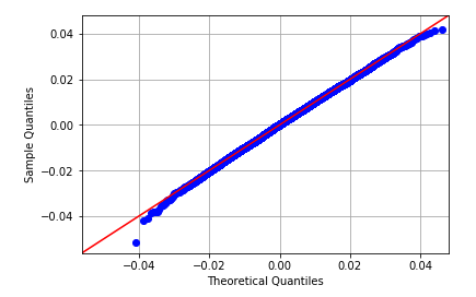
This tendency for mean estimators to tend to a Normal distribution is proven by the Central Limit theorem. So by fitting a Normal distribution, the probability for the estimator to be greater than 0 can be calculated analytically. In this example the Normal distribution is defined by a mean of 0.0026579 and a standard deviation of 0.0166741, which yielded a probability of 59%. If we were to count the number of strictly positive estimator occurrences and divide by our overall estimator sample size, we find a probability of 59.73%. Both results are fairly consistent with one another.

In summary, there is a little more than a 40% chance for this strategy to be a waste of time and risk capital. It seems pretty high for a risk averse trader, but probably quite low for an aggressive speculator. This is where subjectivity kicks in, and everyone will find a level at which they are comfortable operating at.

Conclusion

The percentage number this method generates is a much more intuitive way of appreciating the quality of a trading model than other common metrics like Sharpe Ratio. It can be taken as a basic criterion for quality testing a strategy, simply by comparing its value to a minimum required level. However, it is important to understand and agree with the set of assumptions the final results are based on and also keeping in mind that the larger the original dataset the more reliable the final calculation becomes.

If you like this post, follow me on Twitter and get notified on the next posts.