Further experimentations on the tch-rs crate lead me to explore its use in a Reinforcement Learning setting. In this article, I implement a set of neural networks to find an optimal strategy to a simplified two-player game of Poker using Policy Gradient methods applied to multiple interacting agents. The game in question is a toy version of Limit Hold'em Poker called Kuhn Poker. It can be solved analytically which sets a reference to judge the overall performance of the approach.
Reinforcement Learning framework for Kuhn Poker
If you are unfamiliar with the game, Kuhn Poker requires 2 players and only 3 cards: Jack, Queen, and King. To fully understand the game, please read the short Game Description section in its Wikipedia article. Each player acts in succession, and at each stage, if required, each can choose between 2 different actions. This is the game visualised as the following tree:
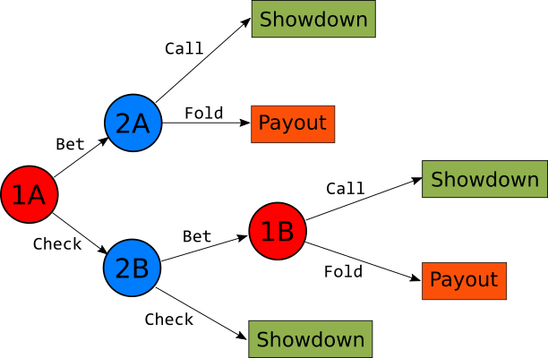
The tree nodes in red represent player1, while those in blue represent player2. The total number of consecutive actions that must be taken in order to get to a final outcome can either be 2 or 3. This is based on the fact that node 1B can only be reached if a Check action and a Bet action have been preliminarily chosen. This means that modelling each player with its own agent requires the current state of the environment to include the actions taken so far. To keep the state definition as simple as possible, I have modelled each node as a single agent and organised them in 2 teams (joint reward). This way, the state variable passed to each agent can be defined by the card held only, and the history of actions only defines whether a particular agent is required to make a choice of not.
Setting up the Torch model in Rust
A natural policy gradient algorithm would only rely on a single policy network per agent, but given that the chosen network architecture could prove difficult to train, adding a network to each agent and estimate a baseline seems a necessary addition. The Vanilla Policy Gradient and Proximal Policy Optimisation algorithms are good candidates and are fairly similar in their implementation, so we will look into setting them up both.
Each agent is then defined by 2 modules that need to be optimised in succession. The easiest way to set this up in the tch-rs crate, is to assign to each module its own VarStore and Optimizer. This way we are sure that all computational graphs in Torch will be handled independently, adding flexibility to the code. For the node 1A for example, it is done as follows:
fn actor1A_builder(p: nn::Path) -> nn::Sequential {
    nn::seq()
        .add( nn::linear(&p / "actor_layer1_1A", 1, 7, Default::default()) )
        .add_fn(|xs| xs.relu())
        .add( nn::linear(&p / "actor_layer2_1A", 7, 2, Default::default()) )
        .add_fn(|xs| xs.softmax(1))
}

fn critic1A_builder(p: nn::Path) -> nn::Sequential {
    nn::seq()
        .add( nn::linear(&p / "critic_layer1_1A", 1, 7, Default::default()) )
        .add_fn(|xs| xs.relu())
        .add( nn::linear(&p / "critic_layer2_1A", 7, 1, Default::default()) )
}

let vs_actor1A = nn::VarStore::new( tch::Device::Cpu );
let vs_critic1A = nn::VarStore::new( tch::Device::Cpu );
let actor1A = KuhnPoker::actor1A_builder( vs_actor1A.root() );
let critic1A = KuhnPoker::critic1A_builder( vs_critic1A.root() );
let opt_actor1A = nn::Adam::default().build( &vs_actor1A, self.lr ).unwrap();
let opt_critic1A = nn::Adam::default().build( &vs_critic1A, self.lr ).unwrap();
The actor and critic neural nets are implemented using a nn::Sequential struct which is itself implementing the nn::Module trait. They are both made up of 2 linear layers connected through a ReLU function. The output of the actor is run through a Softmax function to turn the resulting vector into a multinomial probability distribution.
Model Training
The Vanilla Policy Gradient and the Proximal Policy Optimization algorithms both consist into 2 successive steps:
- Optimising the Policy parameter set in order to maximise a function of the total expected advantage over every batch of trajectories
- Optimising the Value function parameter set in order to minimise the mean error to the collected rewards
The preliminary stage is of course to simulate a batch of trajectories and record all relevant information that need to be subsequently processed by the backpropagation algorithms. While performing these batch simulations, we need to signal to Torch to ignore any gradient calculations as they are not needed at this stage. This is exactly what the tch::nograd function is used for in the code below:
let mut counter = 0;
loop {
  let shuffle = Tensor::of_slice(&[1f32,1f32,1f32]).multinomial(2, false).to_kind(Kind::Float);
  let mut cards : [i64; 2] = [0, 0];
  cards.copy_from_slice( Vec::<i64>::from(&shuffle).as_slice() );

  let state_set = [ cards[0] - 1 , cards[1] - 1, cards[1] - 1, cards[0] - 1 ]; // Center state values around 0

  tch::no_grad( || {

    let probs1A = actor1A.forward( &Tensor::of_slice([state_set[0]]).to_kind(Kind::Float).unsqueeze(0) );
    let probs2A = actor2A.forward( &Tensor::of_slice(&[state_set[1]]).to_kind(Kind::Float).unsqueeze(0) );
    let probs2B = actor2B.forward( &Tensor::of_slice(&[state_set[2]]).to_kind(Kind::Float).unsqueeze(0) );
    let probs1B = actor1B.forward( &Tensor::of_slice(&[state_set[3]]).to_kind(Kind::Float).unsqueeze(0) );

    let action1A = probs1A.multinomial(1, false);
    let action2A = probs2A.multinomial(1, false);
    let action2B = probs2B.multinomial(1, false);
    let action1B = probs1B.multinomial(1, false);

    let actions = [ i64::from(&action1A), i64::from(&action2A), i64::from(&action2B), i64::from(&action1B) ];
    let probs = [ Vec::<f32>::from( probs1A.unsqueeze(0) ), Vec::<f32>::from( probs2A.unsqueeze(0) ), Vec::<f32>::from( probs2B.unsqueeze(0) ), Vec::<f32>::from( probs1B.unsqueeze(0) ) ];
    let rewards = payoff(&cards, &actions);

    for j in 0..4 {
      if rewards[j] != 0f32 { // If reward is zero, the player's action is not relevant to the payoff so ignore it
        let baseline = critics[j].forward( &Tensor::of_slice( &[ state_set[j] ] ).to_kind(Kind::Float).unsqueeze(0) );
        baseline_sets[j].push( Tensor::of_slice( &[ f32::from(baseline) ] ) );
        probs_sets[j].push( Tensor::of_slice( &[ probs[j][ actions[j] as usize ] ] ) );
        reward_sets[j].push( Tensor::of_slice( &[ rewards[j] ] ) );
        action_sets[j].push( Tensor::of_slice( &[ actions[j] ] ) );
        state_sets[j].push( Tensor::of_slice( &[ state_set[j] ] ) );
        if j == 3 { // Counts how many times 1B has played
          counter += 1;
        }
      }
    }
  });

  if counter == min_batch_size { // If player1B has played enough times, exit
    break;
  }
}
In order to simulate a card pick, the multinomial method of the Tensor struct is used, which returns a Tensor representing a sample of indices based on a multinomial probability distribution. These indices represents the cards dealt to each player. The loop is constructed so that it will exit once the most overlooked agent (1B) has been called the minimum number of times set by the user. This ensures that the estimations for this particular agent are statistically relevant.
The next steps are pretty straightforward: The forward function of each Module is called with the relevant recorded state data. Torch starts recording the relevant gradients and an optimisation step can then be launched with the backward_test method of each Optimizer. This function performs the backpropagation and resets the gradient calculation inside the graph to prepare for subsequent calls.
for k in 0..4 {

  let sample_size = reward_sets[k].len() as i64;

  if sample_size > 0 {
    let rewards_t = Tensor::stack( reward_sets[k].as_slice(), 0 );
    let actions_t = Tensor::stack( action_sets[k].as_slice(), 0 );
    let states_t = Tensor::stack( state_sets[k].as_slice(), 0 ).to_kind(Kind::Float);
    let baselines_t = Tensor::stack( baseline_sets[k].as_slice(), 0 );
    let probs_t = Tensor::stack( probs_sets[k].as_slice(), 0 );

    let action_mask = Tensor::zeros( &[sample_size,2], (Kind::Float,Device::Cpu) ).scatter1( 1, &actions_t, 1.0 );

    let probs = ( actors[k].forward(&states_t) * &action_mask ).sum2(&[1], false);
    let advantages = &rewards_t - baselines_t;
    let loss_actor = match algo {
      PolicyGradientAlgorithm::ProximalPolicyOptimisation => -self.ppo_g( &advantages ).min1( &(&advantages * &probs.unsqueeze(1) / &probs_t) ).mean(),
      PolicyGradientAlgorithm::VanillaPolicyGradient => -( &advantages * &probs.unsqueeze(1) ).mean()
    };

    match k {
      0 => opt_actor1A.backward_step( &loss_actor ),
      1 => opt_actor2A.backward_step( &loss_actor ),
      2 => opt_actor2B.backward_step( &loss_actor ),
      3 => opt_actor1B.backward_step( &loss_actor ),
      _ => panic!("Calculation incoherence")
    }

    loss_actors += f32::from(&loss_actor) * 0.25;

    let values = critics[k].forward( &states_t );
    let loss_critic = ( &rewards_t - values ).pow(2f64).mean();

    match k {
      0 => opt_critic1A.backward_step( &loss_critic ),
      1 => opt_critic2A.backward_step( &loss_critic ),
      2 => opt_critic2B.backward_step( &loss_critic ),
      3 => opt_critic1B.backward_step( &loss_critic ),
      _ => panic!("Calculation incoherence")
    }

    loss_critics += f32::from(&loss_critic) * 0.25;
  }

}
Accuracy & Performance
The main problem in this particular setup is having all these agents learning from each other's decisions simultaneously. This intuitively adds risks for oscillations around the optimal results, hence extra risks of divergence. Let's take a look at the training loss charts using the Proximal Policy Optimization approach on 1000 epochs with a minimum batch size of 100:
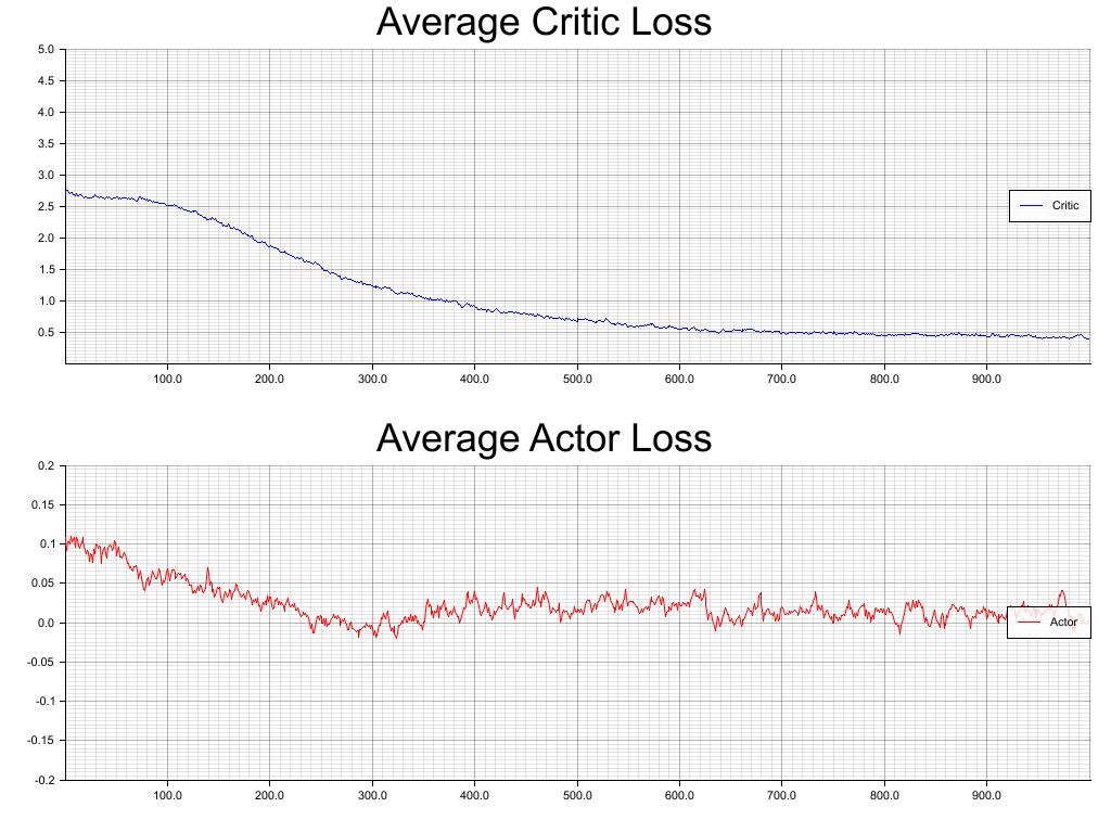
The average loss on the critic modules is converging pretty smoothly while the actor loss seems to be bouncing around a critical level. Let's have a look at the optimal policy derived for each agent and compare it to the analytical solution (a.k.a. Game Theory Optimal):
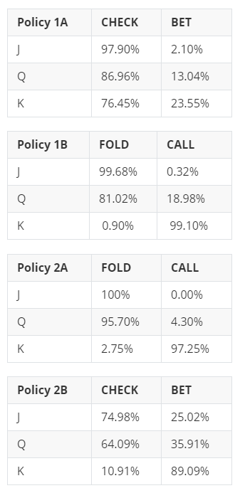
We can see that the model solved the most obvious actions namely, "Always Fold/Never Call with a Jack" as you can never win, and "Always Call/Never Fold with a King" as you can never lose. It is however a mixed success on the more balanced probabilities. Game theory analysis shows for example that player 2B should "Bet with a Jack" 1/3rd of the time, while the algorithm found 1/4th which is not too far but not quite there. It also tells us that player 2A should "Call with a Queen" 1/3rd of the time, while the algo has 1/20th which is a bigger gap.
Conclusion
In order to really understand how precisely the whole network can converge around the optimal solution, further experimentations should be made by adding hidden layers to the neural nets and/or playing around the training hyperparameters. Such investigation is beyond the scope of this article, but if you feel curious about it, feel free to download the Github repo and play around with the code. And of course, do not forget to share if you find more optimal settings...
If you like this post, follow me on Twitter and get notified on the next posts.