In a world where processing power comes in growing abundance, Monte-Carlo methods thrive thanks to their intuitive simplicity and ease of implementation. Over the years, improved versions of the standard Monte-Carlo have emerged reducing the error around the estimate for a given sample size. In this article, we will review the most popular methods and compare their individual efficiency through solving a toy game using Python.
Toy game valuation
Let's first define a simple toy game and solve it analytically. Here are the rules:
-
Throw 2 fair dice and sum their results.
-
The casino pays you the difference between the sum and 8 if it is positive or nothing otherwise.
What is the fair value of the game? Its fair value is the expected value of its payoff. If we call \( S \) the random variable representing the sum of the dice throw, we can derive its distribution by counting the number of occurence of each possible outcome:
| s | 2 | 3 | 4 | 5 | 6 | 7 | 8 | 9 | 10 | 11 | 12 |
|---|---|---|---|---|---|---|---|---|---|---|---|
| p(s) | 1/36 | 2/36 | 3/36 | 4/36 | 5/36 | 6/36 | 5/36 | 4/36 | 3/36 | 2/36 | 1/36 |
Since the payoff function \( f \) of our game can be expressed as:
$$ f \left( s \right) = \max \left( s - 8, 0 \right) $$
We can then easily compute its expected value:
$$ \mathbb{E} \left[ f (S) \right] = \sum_{s=9}^{12} f(s)\ p(s) = \dfrac{5}{9} \approx 0.5556 $$
Let's code this analytical solution in Python:
import numpy

s_values = numpy.arange(2, 13)
s_probas = numpy.concatenate([ numpy.arange(1,7), numpy.arange(5,0,-1) ]) / 36.0

fv = sum( numpy.maximum( s_values - 8.0 , 0) * s_probas )
print(f"fair_value= {fv:.4f}") # fair_value= 0.5556
Before moving on to Monte-Carlo methods, let's define a helper function for printing the mean of a sample and its theoretical standard deviation (see the Central Limit Theorem for more detail)
def mc_summary( xs ):
    N = len( xs )
    mu = xs.mean()
    sigma = xs.std() / numpy.sqrt( N )
    print(f"MC: mean={mu:.4f}, stdev={sigma:.4f}")
Now that we have the analytical answer, let's look into computing the payoff expectation using various Monte-Carlo algorithms and compare their relative performance.
Standard Monte-Carlo
The standard MC algorithm is a direct application of the Law of Large Numbers which states that the mean of the samples of a random variable tends towards its theoretical expected value (unbiased estimator) as the sample size increases.
The standard MC algorithm is simply:
-
Sample \( N \) values of \( S \): \( \{ s_i \}, i \in \{1 \cdots N\} \)
-
Compute the mean of the payoff for each value sampled:
$$ \mathbb{E} \left[ f(S) \right] \approx \dfrac{1}{N} \sum_{i = 1}^{N} f(s_i) $$
Here is the Python code for a sample size of 100k which will be the same across all MC methods:
N = 100000
simulations = numpy.random.choice([1,2,3,4,5,6],size=[N,2]).sum(axis=1)
mc_summary( numpy.maximum( simulations - 8.0, 0 ) ) # MC: mean=0.5584, stdev=0.0033
We find that the theoretical standard deviation of our estimate is around 33bp (bp = basis point). This measurement will be our reference for evaluating the efficiency of the following variance reduction methods.
Control Variate
The first variance reduction method is based around the use of a control variate. The idea is to add to every sample of the payoff function, a corrective term that tracks the deviation from the mean of the sampled variable. The mean of this corrective term tending towards zero, this transformation basically preserves the expectation of the payoff.
Let's write as \( \mu \), the expectation of \( S \):
$$ \mu = \mathbb{E} \left[ S \right] $$
The MC algorithm with control variate is:
-
Sample \( N \) values of \( S \): \( \{ s_i \}, i \in \{1 \cdots N\} \)
-
Compute the mean of the payoff for each value sampled:
$$ \mathbb{E} \left[ f(S) \right] \approx \dfrac{1}{N} \sum_{i = 1}^{N} \left[ f(s_i) + c \left( s_i - \mu \right) \right] $$
where \( c \) is chosen as opposite to the correlation between \( S \) and \( f(S) \)
We choose the coefficient \( c \) that minimises the standard deviation of the estimate:
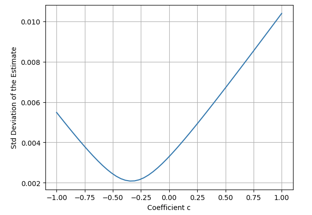
The implementation of the algorithm in Python is very straightforward:
mu = numpy.sum( s_values * s_probas )

mc_summary( numpy.maximum(simulations - 8.0, 0) - 0.3 * ( simulations - mu ) ) # MC: mean=0.5555, stdev=0.0021
Antithetic Variate
The antithetic variate method consists in replacing the payoff function computed for a sampled outcome with the average with its computed value for an outcome chosen on the other side of the mean and of the same probability as the original sampled outcome. This way, the expected payoff estimation is again preserved in the tranformation.
The MC algorithm with antithetic variate is:
-
Sample \( N \) values of \( S \): \( \{ s_i \}, i \in \{1 \cdots N\} \)
-
Compute the mean of the payoff for each value sampled:
$$ \mathbb{E} \left[ f(S) \right] \approx \dfrac{1}{N} \sum_{i = 1}^{N} \dfrac{f(s_i) + f(\bar{s}_i)}{2} $$ where \( \bar{s}_i \) is the symmetrical value to \( s_i \) on the other side of the mean
The implementation of the algorithm in Python in our case is also very straightforward:
antithetics = 14 - simulations

mc_summary( 0.5 * ( numpy.maximum( simulations - 8.0, 0 ) + numpy.maximum( antithetics - 8.0, 0 ) ) ) # MC: mean=0.5546, stdev=0.0020
Importance Sampling
We can gain an intuition around this next technique by reasoning about the toy game in the following manner. Since the payoff is zero for a large subset of the final outcomes \( (s \leq 8) \), the contribution of these to the calculation of the average payoff is less than those that generate a strictly positive value. So, could we sample more of these meaningful values while preserving the mean estimate? This is what importance sampling effectively does. We define a new random variable covering the same outcomes as our original one, but with a distribution skewed towards outcomes of interest.
Mathematically, let's define the random variable \( X \) defined on the same measurable space than \( S \) but where the probability for a strictly positive payoff is much larger than the probability of a payoff equal to zero:
| x | 2 | 3 | 4 | 5 | 6 | 7 | 8 | 9 | 10 | 11 | 12 |
|---|---|---|---|---|---|---|---|---|---|---|---|
| p(x) | 1/35 | 1/35 | 1/35 | 1/35 | 1/35 | 1/35 | 1/35 | 7/35 | 7/35 | 7/35 | 7/35 |
Using a change of measure from \( S \) to \( X \) we can write:
$$ \mathbb{E}_S \left[ f(S) \right] = \mathbb{E}_X \left[ \dfrac{f(X)\ p_S(X)}{p_X(X)} \right] $$
The MC algorithm with importance sampling with respect to \( X \) is:
-
Sample \( N \) values of \( X \): \( \{ x_i \}, i \in \{1 \cdots N\} \)
-
Compute the mean of the payoff for each value sampled:
$$ \mathbb{E} \left[ f(S) \right] \approx \dfrac{1}{N} \sum_{i = 1}^{N} \dfrac{f(x_i)\ p_S(x_i)}{p_X(x_i)} $$
Its Python implementation requires slightly more variable definitions but still remains fairly concise:
x_probas = numpy.concatenate([ numpy.ones(7) / 35.0, numpy.ones(4) * 7.0/35.0 ])
p_s = numpy.vectorize( lambda x: s_probas[ s_values.tolist().index(x) ] )
p_x = numpy.vectorize( lambda x: x_probas[ s_values.tolist().index(x) ] )
simulations_x = numpy.random.choice(s_values, size=N, p=x_probas)

mc_summary( numpy.maximum( simulations_x - 8.0, 0 ) * p_s( simulations_x ) / p_x( simulations_x ) ) # MC: mean=0.5552, stdev=0.0010
Stratified Sampling
This last method consists in drawing a random variable from different subsets of outcomes while preserving its mean by adjusting the frequencies of draws from each subset. It follows in the steps of importance sampling but goes even further because it allows us to arbitrarily choose subsets that simplify the resolution of our specific case.
For our toy game, we can choose to only draw from the subset of outcomes larger than 8 since all the others have a payoff of zero, and as such do not contribute any value to the calculation of the average.
Mathematically, let \( Y \) be the set of the value of \( S \) greater than 8. Since the payoff function is equal to 0 for any value of S not contained in \( Y \), by the Law of Total Expectation, we can write:
$$ \mathbb{E} \left[ f(S) \right] = \mathbb{E} \left[ f(Y) \vert Y \right]\ \mathbb{Pr} \left( Y \right) $$
We can easily compute:
$$ \mathbb{Pr} \left( Y \right) = \dfrac{4 + 3 + 2 + 1}{36} = \dfrac{5}{18} $$
We compute the conditional density with respect to \( Y \):
| y | 9 | 10 | 11 | 12 |
|---|---|---|---|---|
| p(y) | 2/5 | 3/10 | 1/5 | 1/10 |
The MC algorithm with stratified sampling with respect to \( Y \) is:
-
Sample \( N \) values of \( Y \): \( \{ y_i \}, i \in \{1 \cdots N\} \)
-
Compute the mean of the payoff for each value sampled:
$$ \mathbb{E} \left[ f(S) \right] \approx \dfrac{1}{N} \sum_{i = 1}^{N} f(y_i)\ \mathbb{Pr}\left( Y \right) $$
Another very succinct Python implementation:
y_values = numpy.arange(9,13)
y_probas = 0.1 * numpy.arange(4,0,-1)
simulations_y = numpy.random.choice(y_values, size=N, p=y_probas)

mc_summary( ( simulations_y - 8.0 ) * 5.0 / 18.0 ) # MC: mean=0.5560, stdev=0.0009
Conclusion
Here are the improvements in standard deviations of the estimated expected payoff in our toy game and for all methods reviewed. The standard MC value is used as reference:
The level of performance can be divided into two distinct groups: The control variate and antithetic variate methods in the first, and importance sampling and stratified samping in the other. The latter group which implements an actual distribution adjustment achieves far better variance reduction overall.
For path dependent cases and complex payoffs, efficiently applying these variance reduction techniques can be more challenging. However, trying and fine-tuning different approaches often leads to finding a decent solution.
If you like this post, follow me on Twitter and get notified on the next posts.